Chapter 6 Calculation
MongoDB has two methods for performing in-database calculations: aggregation pipelines and mapreduce. The aggregation pipeline system provides better performance and more coherent interface. However, map-reduce operations provide some flexibility that is not presently available in the aggregation pipeline.
6.1 Aggregate
The aggregate() method allows you to run an aggregation pipeline. For example the pipeline below calculates the total flights per carrier and the average distance:
stats <- flt$aggregate(
  '[{"$group":{"_id":"$carrier", "count": {"$sum":1}, "average":{"$avg":"$distance"}}}]',
  options = '{"allowDiskUse":true}'
)
names(stats) <- c("carrier", "count", "average")
print(stats)
#> carrier count average
#> 1 OO 32 500.8125
#> 2 F9 685 1620.0000
#> 3 YV 601 375.0333
#> 4 EV 54173 562.9917
#> 5 FL 3260 664.8294
#> 6 9E 18460 530.2358
#> 7 AS 714 2402.0000
#> 8 US 20536 553.4563
#> 9 MQ 26397 569.5327
#> 10 UA 58665 1529.1149
#> 11 DL 48110 1236.9012
#> 12 B6 54635 1068.6215
#> 13 VX 5162 2499.4822
#> 14 WN 12275 996.2691
#> 15 HA 342 4983.0000
#> 16 AA 32729 1340.2360Let’s make a pretty plot:
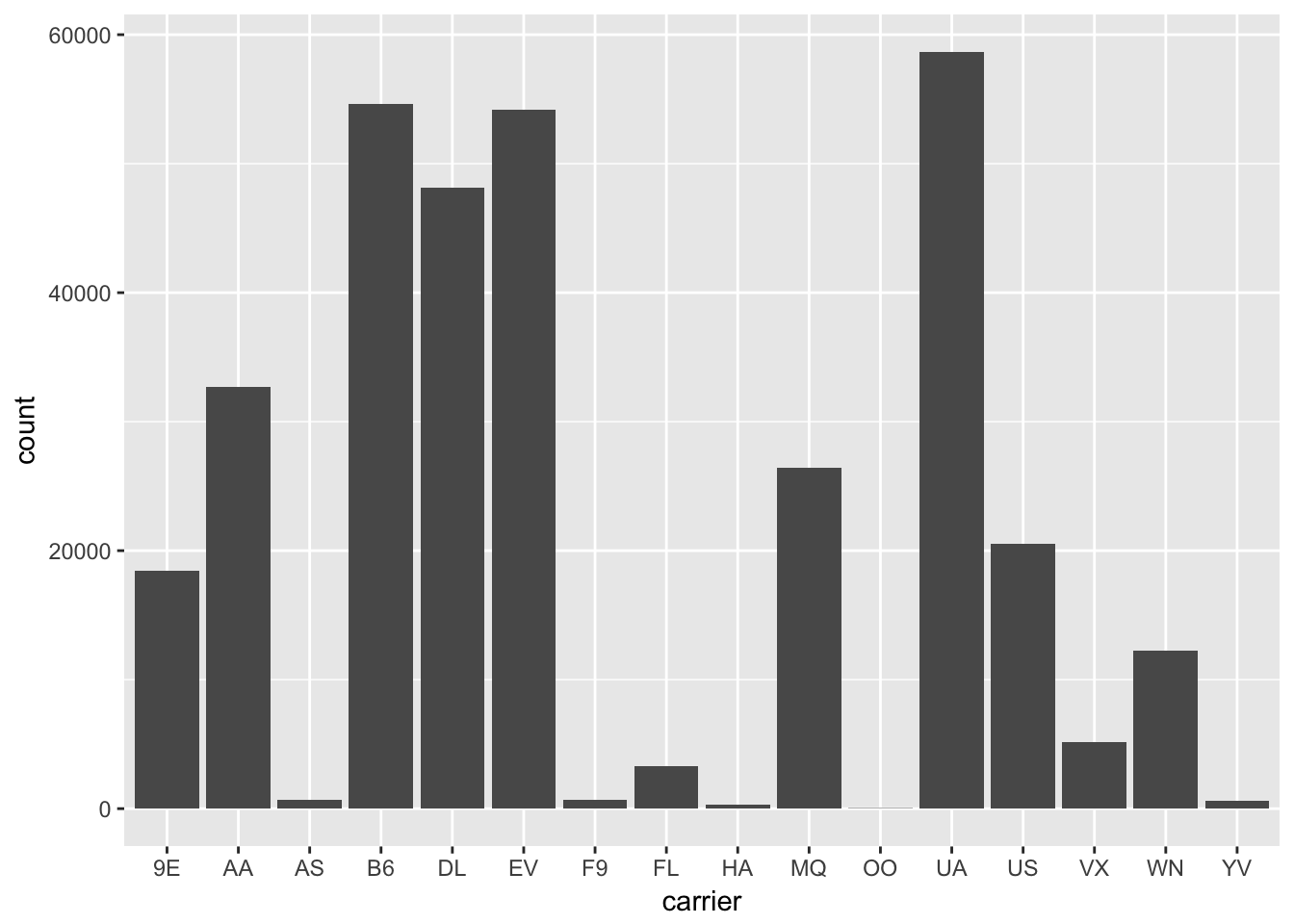
Check the MongoDB manual for detailed description of the pipeline syntax and supported options.
6.2 Aggregation Iterators
If you are expecting a lot of data or do not want to automatically simplify the results into data frames, run the aggregation with iterate = TRUE:
iter <- flt$aggregate(
  '[{"$group":{"_id":"$carrier", "count": {"$sum":1}, "average":{"$avg":"$distance"}}}]',
  options = '{"allowDiskUse":true}',
  iterate = TRUE
)
This will return the results in the form of an iterator just like when using the iterate method. You can then iterate over the results one by one or in pages:
#>  [1] "{ \"_id\" : \"OO\", \"count\" : 32, \"average\" : 500.8125 }"
#>  [2] "{ \"_id\" : \"F9\", \"count\" : 685, \"average\" : 1620.0 }"
#>  [3] "{ \"_id\" : \"YV\", \"count\" : 601, \"average\" : 375.033277870216 }"
#>  [4] "{ \"_id\" : \"EV\", \"count\" : 54173, \"average\" : 562.9917301977 }"
#>  [5] "{ \"_id\" : \"FL\", \"count\" : 3260, \"average\" : 664.829447852761 }"
#>  [6] "{ \"_id\" : \"9E\", \"count\" : 18460, \"average\" : 530.235752979415 }"
#>  [7] "{ \"_id\" : \"AS\", \"count\" : 714, \"average\" : 2402.0 }"
#>  [8] "{ \"_id\" : \"US\", \"count\" : 20536, \"average\" : 553.456271912739 }"
#>  [9] "{ \"_id\" : \"MQ\", \"count\" : 26397, \"average\" : 569.532712050612 }"
#> [10] "{ \"_id\" : \"UA\", \"count\" : 58665, \"average\" : 1529.11487258161 }"
6.3 Map/Reduce
The mapreduce() method allow for running a custom in-database mapreduce job by providing custom map and reduce JavaScript functions. Running JavaScript is slower using the aggregate system, but you can implement fully customized database operations.
Below is a simple example to do “binning” of distances to create a histogram.
# Map-reduce (binning)
histdata <- flt$mapreduce(
  map = "function(){emit(Math.floor(this.distance/100)*100, 1)}",
  reduce = "function(id, counts){return Array.sum(counts)}"
)
names(histdata) <- c("distance", "count")
print(histdata)
#> distance count
#> 1 0 1633
#> 2 100 16017
#> 3 200 33637
#> 4 300 7748
#> 5 400 21182
#> 6 500 26925
#> 7 600 7846
#> 8 700 48904
#> 9 800 7574
#> 10 900 18205
#> 11 1000 49327
#> 12 1100 6336
#> 13 1200 332
#> 14 1300 9084
#> 15 1400 9313
#> 16 1500 8773
#> 17 1600 9220
#> 18 1700 243
#> 19 1800 315
#> 20 1900 2467
#> 21 2100 4656
#> 22 2200 5997
#> 23 2300 19
#> 24 2400 26052
#> 25 2500 14256
#> 26 3300 8
#> 27 4900 707From this data we can create a pretty histogram:
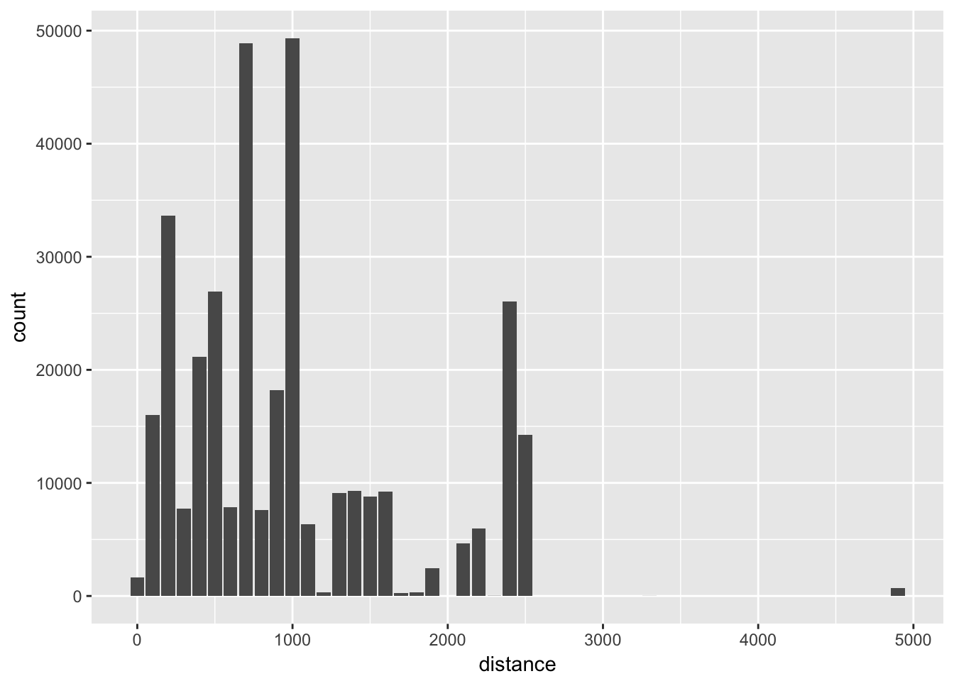
Obviously we could have done binning in R instead, however if we are dealing with loads of data, doing it in database can be much more efficient.